
|
Today we will be looking at the Page Layout Tab in
Microsoft Excel 2007. This Tab has many new features
that will let you change the look and feel of your Excel
workbook. The Page Layout Tab is divided into the
following groups:
Here is a screen shot of the Page Layout Tab in Microsoft
Excel 2007.
|

|
Themes Group:The first group that we will look at is the
Themes group. Themes in Microsoft Excel provide a unique
and professional look to your Workbooks. They can do
this by using an assortment of font styles, color schemes and
graphical effects.
We will use a customer list
workbook for our lesson today. I have included a screen shot of
our data in the figure below. We have some basic
information on our customers like first names, last names,
addresses and the phone numbers. Notice that we do not
have any formatting applied to it yet and it looks rather
plain and simple.
Before you can use
Themes, you need to apply a little formatting to some of your
data elements. In our case, we would like to use a
Title and also emphasize or Column Headings. We also need to change the
row height to 30 pixels to accommodate the bigger
Title. We can do that by clicking on row header of
the first row. Then we browse onto the Home Tab in Excel
2007 and choose Cell Styles command in the Styles
group. We would like to change the text Customer
Master List to
Heading 1.
The specific
steps are highlighted below in the screen shot.
|

|
Moving onto the column headings, we need to make them
prominent as well. We will again use Cell Styles command
from the Home Tab and then select custom formatting style
something like Good .
The last action and its effect is illustrated
in the figure below.
|

|
Now we are
finally ready to experiment with Themes in Microsoft Excel
2008. I have moved your title Customer
Master List to cell D1 so it is positioned in the center.
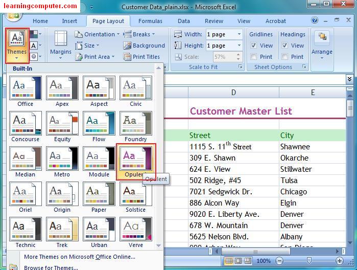
Using the Page Layout Tab, click on Themes drop down
in the Themes group. You will get a host of built-in,
pre-defined and ready made available Themes. Notice
as you browse from one option to another, Microsoft Excel
will not only change the underlying format but also give you
a live preview of the end result, Very Nice
Indeed!
We will go ahead and choose Opulent for our
theme choice. Here is what this step looks
like.
|
|
If you are not
happy with the color scheme, you can certainly use one of the
many available Theme Colors from the Themes Group. For
our customer list, we would like to use maybe
Equity
since this color scheme is more
professional looking.
Notice below that using the
Theme Colors will not affect the font style, just the font
color.
|

|
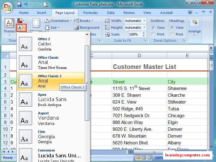
The last
option we'll cover in the Themes group is to use one of the
Theme Fonts from the drop down list. We would like to
emphasize the Title and Heading elements a little more in our
customer list. Using the Theme Font functionality, we
can possibly choose Office Classic 2.
As we hover the mouse over the Theme Fonts, we
get a Live Preview of its effect on our
Worksheet.
|
|
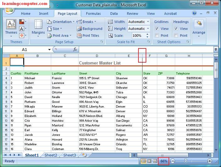
The final version of our document is shown below. I
have changed the Zoom Level to 66% so you can see the
data a bit better and also to include all the data
columns.
Here is the screen capture. Notice the
dotted line after column E, this is where is Excel workbook
will be split into two pages when printed.
|
|
Page Setup group: Moving onto the next group, here we have many
different choices for our Microsoft Excel worksheet
layout. Let us take a look at these one at a time.
First of all I would like to change your view from
Normal to Page Layout so I can see the effect of your Page Setup
choices clearly. I can do this by selecting the View
Tab on the Ribbon and then choosing Page Layout
option.
The command and its effect are shown
below. The Page Layout shows us the worksheet in
its printed form which was sometimes a challenge in the
past. We can now see the margins on all sides, the header
block and all the column headings that will be included in the
first page.
|

|
The first Page Setup option is Margins, which
lets you control the white space in your document. We
would like to switch margins in the worksheet from Normal to
Narrow so we can see more of customer data when we print this file.
Go ahead and click on Margins command and then select Narrow
from the drop down menu.
This action is
highlighted below from your
computer monitor.
|

|
You will see
that there is less space on the right and left sides of your
worksheet now. As a result of this, now we can even see the
State column on your first page as shown below,
Cool!
|

|
The next
command is Orientation under the Page Setup Tab in Microsoft Excel
2008. This will let you toggle between Portrait
and Landscape views for printing purposes.
Currently we are using
Portrait view. Lets us switch it to Landscape view
by clicking on Orientation drop down and then choosing Landscape.
After this action, you will be able to see all
the columns in your Excel Sheet. Go ahead and click Save icon on Quick Access
Toolbar. The next two screen capture hight light the effect of
using Landscape Orientation.
|

|

|
You can
further fine tune some of the print settings also. You can either use the Page Setup
button either from the Print Preview screen or by using Dialog
box launcher button (small red square) in the bottom right corner of
Page Setup group on Page Layout Tab,
Here is a screen shot
of the Page Setup dialog box. For now I am going to switch
back to Portrait and then click Ok.
|

|
|
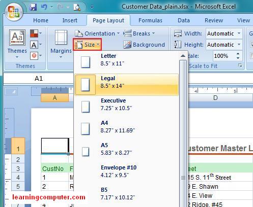
Using the Size command is pretty handy if you
need to do some specialized paper printing. Let's assume
that you would like to print customer data to a legal format as opposed
to a letter format. You can easily do this by selecting
Size command and then choosing an Legal from the
list.
The screen capture below highlights this
change in Paper size.
|
|
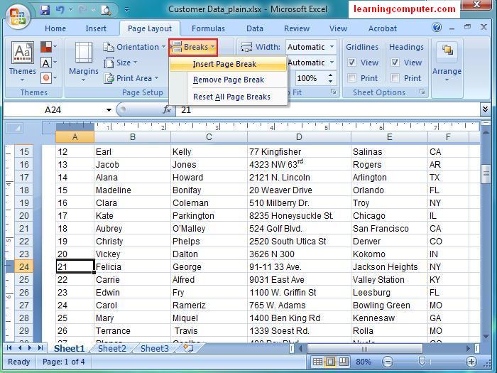
What if you wanted to insert a page break lets say
after the first 20 customers? You can easily do this
by moving your mouse to the 21st customer, clicking on
Breaks command and then choosing Insert Page Break.
Here's the illustration of the necessary
steps.
|
|
The next
command is Background on the Page Setup Tab and
it will let you add a background image to your Excel
workbook. This could be beneficial if you are trying to
insert possibly the company logo with your data.
When you click on this command, it will give you a new
dialog box where you can select the picture and then click OK.
We will proceed onto the next feature.
The Print Titles
command is quite essential when you are trying to print a lot
of information that spans multiple pages. This
scenario does apply to our current customer list as it
spans over four pages.
Before we try this option, let us do you a
Print Preview using the Office button. When I did this,
notice the first page has all the column headings,
however they are missing from the second
page, definitely not good!
This is visible in the screen shot right
below.
|

|
You can easily fix this problem by using the Print
Titles command. When you click on this command, you get
the Page Setup dialog box we have already seen
before.
Go ahead and select the icon under
Rows to repeat at top. Here is the
associated screen shot.
|

|
Next browse back to the first row (3) and select all the
row headers. This will insert the necessary information
in the Page Setup dialog box. Go ahead and click
OK. We have included the related screen
capture.
|

|
Now when you do a final Print Preview, the column headings
do show up on the subsequent pages, very nice indeed.
The the column headings on the second page are shown
below.
|

|
|
Scale to Fit
Group:
For the next set of exercises that switch back
to the portrait view. When we did that notice that the
column Headings after City are now spanning over to the next
page on the right. How can we fix this?
We can take care of this by using the Scale
to Fit group. Under the Width command, click on the
drop down and select 1 page.
|
|
Now when I do Print Preview, it adjusted the
formatting so that all the columns fit onto one page as
shown below, Sweet!
|

|
In a similar fashion, you can also control the height
of your Excel Sheet. Under the Height command, you can select
1 page option. This will change the formatting scale of
your data to fit it on 1 page.
When I did a Print
Preview again, now the customer data is looking rather small. I
will then switch it back to 2 pages for the Height,
as illustrated below.
|

|
When
we did a final Print Preview, everything look great. If you notice on the
bottom left corner in the Status Bar, we have now shrunk the
data to 2 pages instead of 4. Let us go ahead and save the
file now.
|

|
Sheet Options
Group:
The next group we will go over is Sheet Options. We have
two properties that we can control here, Gridlines and Headings.
Currently they both are checked and this is also shown
in the Microsoft Excel sheet below.
|

|
First let us
see the effect of removing Gridlines. You can simply uncheck the View box
under the Gridlines menu. This will yield a much cleaner format
of your data as the gridlines have been removed.
Here is
what it looks like.
|

|
In the
second step, you can go ahead and uncheck the View box under Headings Menu.
Notice that it removed both the row and column headings after
this action. This also gives you more real estate and shows
a little more of your datasheet than before.
Here is a
screen capture of removing the Headings.
|

|
Arrange Group:
The last group in the Page Layout Tab is Arrange. This
is primary used with pictures or images. Once you have
such an element in your workbook, you can then use Arrange
commands to position the item relative to your data. For now
we will skip over this and come back to it when we go over the
Insert Tab.
|
Related Links:
Access 100's of video training courses for Free!!
http://office.microsoft.com/en-us/excel/HA100215631033.aspx
http://www.viu.ca/technology/docs/Quick_reference_excel_000.pdf
http://news.office-watch.com/img.aspx?img=902-Excel%202010%20TP%20-%20Page%20Layout%20tab.jpg&a=902
|
|
