|
Excel Formulas Tab
The Formulas Tab
in Microsoft Excel 2007 greatly simplifies the task of number
crunching. The Excel Formulas Tab has the following
groups:
Before we
get started with the Excel Formulas Tab,
let's talk about basic math, functions and formulas. In
order to
show you basic Math operations, I have copied a list from Microsoft
office help. This table shows you the basic math
operator symbols, their meaning along with examples. These
will come in handy as we work with data in our
lesson on Excel Formulas today.
|
Arithmetic operator |
Meaning |
Example |
|
+
(plus sign) |
Addition |
3+3 |
|
(minus sign) |
Subtraction
Negation
|
31
1 |
|
*
(asterisk) |
Multiplication
|
3*3 |
|
/
(forward slash) |
Division
|
3/3 |
|
%
(percent sign) |
Percent
|
20% |
|
^
(caret) |
Exponentiation |
3^2 |
In Microsoft Excel
2007, mathematical computations are typically done by built-in
functions. Excel has a library of several hundred
functions on Formulas Tab that will let you perform a
number of mathematical and statistical calculations.
For example you can use the sum function to add numbers,
average function to compute averages on a list of numbers, the PMT
function to figure out payment on a loan, so on and so forth.
In order to use these functions, we need
to have some basic knowledge about the underlying
formulas. Microsoft Excel 2007 does a great job of filling in the
blanks, however it is vital that you have some understanding
of these basic concepts. Excel uses the values from
cells (cell referencing) to compute the end result using
formulas and functions.
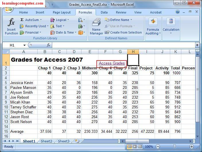
Let's go ahead and see the function
capabilities of Excel 2007 Formulas Tab in action
next. We are going to be using a Grading workbook for
our lesson today. We have the students listed on the left
side while the assignment and test scores are noted across the
columns. I have included a screen shot of
the students grades data here with the Excel Formulas
Tab highlighted in red.
|

|
We will
start with the AutoSum command on
the Functional Library group under the
Formulas Tab in Microsoft Excel. We would like to know the
total scores achieved by every student across all the assignments and
tests. We have designated column K (Total) for the total
scores. Go ahead and click on the cell K6 which would
highlight Jessica Kevin's total points. Click on AutoSum command
on the Ribbon under excel formulas tab as shown in the
screen capture below.
|

|
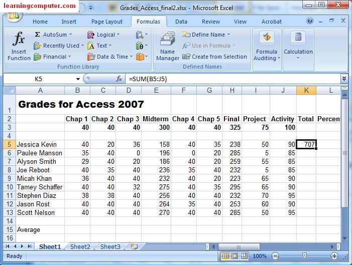
You will
notice that Microsoft Excel placed a dotted rectangle around
the cells from B5 through J5. In addition it placed this
function =Sum(B5:J5)
in cell K5. Notice that all
functions in Excel start with an equal sign. What this
function is saying is that we would like to add all the
numbers from B5 through J5 and place the result in cell
K5.
After I
pressed the Enter key, Excel 2007 computed the result and placed the total score
of 707 in the correct location as visible below.
|
|
This is
great, but how can we
copy this formula to the other students data? Let's see that
in our next practice on Excel Formulas Tab. We are
going to use the copy formula ability in Microsoft Excel
2007 to repeat this task. Select cell K5, and move the mouse
to the right bottom quarter of the cell until the icon changes
to a fill handle. Holding the left mouse button, you
cannot drag your mouse all it down to cell K13 and then let go
of the mouse.
This action
under Formulas Tab in Microsoft
Excell is shown below.
|

|
It will go
ahead and sum
up the scores for all the students just like it did for
Jessica Kevin. Very nice! If you prefer using the
keyboard you could've done the same thing by using copy (Ctrl+C)
and paste (Ctrl+V) commands.
|

|
Next we
would like to compute the Average for
all the class assignments and the test scores. We'll
be adding this information in row 15. Go ahead and
click on cell B15. This time we are going to click on
the Excel Formulas Tab and select Insert Function
command
which will launch Insert function dialog box as shown below.
|

|
Go ahead and type Average in the search
text box and then click OK. You will get the
Function Arguments dialog box next. Microsoft Excel 2007 is smart enough to
pick cells B5 through B14 (adjacent cells), the scores for
Chapter 1 assignment. You can see some additional information
on this dialog box. It even has a links to the Excel Help section if
you need more explanation. Finally hit OK on this one.
|

|
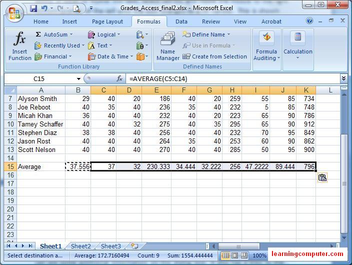
Observe that
it went ahead and computed the average (37.55) and placed the
end result in cell B15, Sweet!
You can see how easy it is to
work with functions and formulas in Microsoft Excel 2007. We are
going to copy the average formula to all the other class
assignments and tests. Instead of dragging the fill
handles, go ahead and select the B15, do right
click on the mouse and choose Copy. This will copy the
formula to the clipboard and place dotted borders around the
cell. Next hold the left mouse
button and select cell C16
through K16. Finally choose paste from the
right click menu.
I have included these action
and its effect in the following two figures
on Microsoft Excel Formulas Tab.
|

|
|
|
Our Excel
Grade Worksheet is looking pretty good so far and giving us
some meaningful results about our students grades. We
need to do one more thing which is to calculate the percentage
of every student in the last column L. However let's
take a look at some of these other commands on the
Function Library on Excel
Formulas Tab
first.
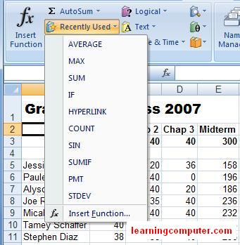
Right next to the
AutoSum command, we have a list of Recently
Used
functions. This comes in
handy when you are using a few functions over and over
again. In our case when I selected the dropdown, I was
able to see the following functions.
|
|
The next few
commands include functions that relate to a specific
category. The Financial drop down has a
host of functions like loan, interest, security etc.
Logical functions include operators like
true, and, or and if. Text functions
are useful to perform operations like converting text case,
replacing text, concatenation and string manipulation. The
next command is definitely beneficial as it has to do with
Date & Time functions in
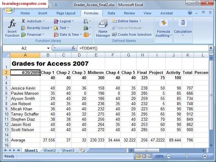
Excel Formulas Tab. Maybe we can
try an example from this one. Let's say that we would
like to add today's date in our Excel Sheet. How can be we do
this task?
Go ahead and select cell A2,
click on the Date & Time
command and select
Today from the list. Bingo! The next two screen captures
display this functionality.
|

|
|
|
The next
function command under Excel Formulas
Tab is Lookup &
Reference. This one has a few useful options;
hyperlink is the one that I tend to use sometimes. Let
me show you how this one works next.
Let's say
that we need to store our Grading Excel sheet somewhere on
the network, possibly for your co-workers to look at the
data. We can use the hyperlink command to achieve
this. Select the cell F1 as the location where we would
like to insert the hyperlink. Choose Hyperlink from
the Lookup & Reference drop down as shown
below.
|

|
Next you will get the Function
Arguments dialog box shown in the first screen shot.
For the link location, enter a value similar to this
one:
C:\Users\kmughal\Documents\Grades_Access_final2.xlsx
For
the friendly name, enter Access Grades and then click
OK.
In the second screen shot, you will observe
that now we have a hyperlink (cell F1) to this file so when I
email this to my colleague, he/she can go to the original file
by clicking on this link. In this manner, if the underlying
data has been updated, they can simply go to the most recent
version!
|

|
|
The next
function command is Math & Trig which includes quite a
few mathematical function and formulas in Excel 2007. The
last listed option is More Functions
. When I selected this dropdown, the choices that
I see are listed below.
|

|
We are finally done
with the Functions Library which as we have seen is quite
elaborate in Microsoft Excel 2007. We can move onto of the
next group of commands which is Defined
Namesunder Excel
Formulas Tab.
Utilizing a named cell or range
of cells can make your Excel Workbook more
personalized. Let's see how we can do this in the next
practice. Please note that cell K3 has the maximum
possible points (1000) for our Access 2007 class.
We would like to use a Name for this value so we can use it to
compute the students percentages in the next section.
Select cell K5, then click on Define
Name under the Defined Names
group. This will invoke the New Name dialog box as shown
below. For name enter Total_Points, add any additional
information and then click OK. Now we are able to
use this name cell in our Class Percentage
formula.
|

|
|
We need to
find the overall percentage received by every student. This is
necessary so we can find out the final grade. Go
ahead and click on cell L5. Type in this formula
=K5*100/to. You will notice that after
you type to, you now get an option for Total_Points. Go
ahead and select this to complete the percent formula which
will be=K5*100/TotalPoints.
There's an excel
formulas tab
screen shot of this step and resulting percentage are shown as
follows.
|

|

|
As a final
step in this group, we need to copy
this percentage to all of the other student scores as well. This time
let us try using the keyboard. First you need to select cell L5, press control
+ C, click on cell L6 and holding down the Shift key and
go all the way down to L15 by using the down arrow key. Finally
do Control + V to paste the formula in the new
cells.
|

|
The next two groups
Formula Auditing and
Calculation are really more for advanced
topics so we will go over only a few
options.
Sometimes when your worksheet gets really crowded under Excel
Formulas Tab, it helps to have some sort of navigation for
all your formulas and functions. Our grade book is
fairly simple so this is not the best example for
this. But let's say we wanted to know
where are total scores and averages coming from? We
could select cell B15 and click on Trace
Precedents. This will highlight all the cells that are
being used to compute the Average which is the value in cell
B15.
This is what it looks like on my computer
display.
|

|
In a similar
fashion we can also
find out dependents in my Excel Workbook. For example I
am curious to find out if any cells are using the
value from cell E5. I click on that cell and then
select Trace Dependents on Excel Formulas Tab. This will
highlight cells K5 and E15 as highlighted below. What this
means is that the cells K5 and E15 (Total and Average) depend
on E5 for its computation.
|

|
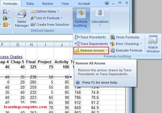
If you want to
remove all the precedents and dependents from your Excel
Workbook, you can simply use Remove Arrow under the Formula
Auditing group. This will clear all the arrows from your
worksheet.
|
|
Last but not
least, a useful command in this group
is the Show Formulas command on Microsoft Excel
Formulas Tab.
Sometimes it makes sense
to locate all the formulas in your Microsoft Excel
2007 worksheet, maybe you need to print it out for your
reference. You can do this by using Show Formulas command
under the Formula Auditing group. When I did this on my Excel
sheet, this is what I saw. Notice you have one central place
where you can review all the functions and formulas. Lets go
ahead and save the spreadsheet now.
|

|
Other Useful links on Excel Formulas Tab
-Excel
Formulas and Functions
-Access 100's of video training courses for Free!!
-Excel
Formulas and Functions
-Microsoft
Excel Formulas
-Excel
2007 Training Video
-Excel
2007 User interface Formulas Tab
|
|
This concludes the
tutorial on Microsoft 2007 Excel Formulas Tab.
|
