|
In our lesson
today on Microsoft excel office , we will be looking at the Data Tab in
Excel 2007. Using this tab, you can import data
from external sources including but not limited to a text
files, Microsoft Access databases, web pages, xml documents,
Microsoft Query, Microsoft SQL Server databases. We will
show you how to import data from a Microsoft Access
database and also from a text file.
The data
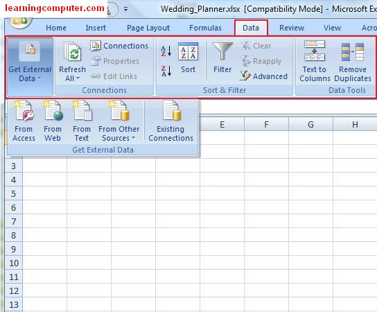
tab has the following groups that you can utilize:
Get External Data Group
Connections Group
Sort & Filter Group
Data
Tools Group
Outline Group
Here is a screen shot of the Data Tab in
Microsoft Excel 2007.
|
|
Get External
Data
:
Go ahead and
launch Microsoft Excel and open up a new workbook using
the Office button. Next select From Access command on
the Get External Data group. When you click on this, a
new dialog box will pop up. Select your data source
which will be a Microsoft access database and then click
Open.
For our practice today, we'll be using a wedding
database (Wedding.accdb) from My Documents folder. We
have included a screen capture of this step
right below.
|

|
Next you will
get the Select Table dialog box where you can choose the actual table.
We will choose Expenses table from the wedding database
and then click OK. This action is shown as follows.
|

|
After you
click OK, another next dialog box titled Import Data will pop
up. This is where you can select what type of data will
you be using for the import. In addition you can choose the location in
your worksheet where you would like to place the
imported data.
We will just select Table and Existing
worksheet (cell A1) as our choices.
|

|
Microsoft Excel 2007 will go ahead and imported the data into our existing
worksheet now. In addition the imported data came in as
an Excel table format. An Excel table
automatically provides you some nice graphical effects along with
a header row with built-in filtering capabilities.
You can see the header row in blue
background with drop down arrows in the figure
below. This Excel table is independent of the data
in rest of your Excel sheet. We will come back to this
wedding data in a bit.
|

|
Let's try to import more data into our Excel
workbook, this time maybe using a text file. We have a
customer list on our computer in the form of a text file and would like
to get this information into Microsoft Excel 2007.
This time choose From Text on the Get External Data group.
Included is a display of this steps from our computer
screen.
|

|
Next you
will get the Import Text
File dialog box shown as follows. Go ahead and select the
customers file while is Customers.txt in our case. Lastly click
on Import.
|

|
This process
will start the Text Import Wizard
which will guide you through the data import process. In step
1, the wizard will try to figure out if you are
using data in fixed width or delimited format. Our text file is in
delimited format so we will choose that
option as shown below.
After that go
ahead and click Next .
|

|
|
In Step 2 of the wizard, you can choose what type
of character is being used for delimiting the data. In
our case we are using comma, so we will go ahead
and select Comma check box. This Delimiter choice is also
validated in the Data preview pane which it looks good. Go ahead and click
Next.
This is captured by the monitor screen shot
right here.
|

|
In the
final step of the wizard, you can select the data type
for each of the fields that you are
importing. A data type defined what type of information is being
used in a column or field. The wizard recommends General as
a good choice so we will pick this setting for all
of our columns to keep things simple.
Here
is what this step looks like an action.
|

|
The
last piece of information the wizard wants to know is the
location of this customer data. We will select Existing worksheet
with cell A1 as our location. Finally we will hit OK to
start the actual import process.
|

|
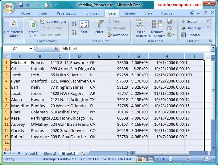
The wizard
was successful in importing the customer data to our Excel
workbook as shown in the figure below.
The first row has
all the correct column headings like FirstName, LastName, Address information etc.
In addition notice that this data is in
Sheet 2 of our workbook.
|

|
Connections
Group
:
Moving onto the next group which
is Connections
. When I clicked on this
command it brought up a dialog box titled Workbook
Connections. This is shown in the screen capture
below.
You will see that both
of our imported files, Wedding (from Access database) and Customers
(text file) are listed here. This is also where you can
set additional properties of your data sources and refresh them if you
like.
|

|
Sort & Filter
group
:
The next
group of commands falls under the Sort and Filter group as
highlighted below.
Using this tab, you can sort
and filter your data on one or more columns. Let us
say that we want to sort the wedding expenses information
by the CategoryLookup column in an ascending order. You
can select that column and then click on the first icon which
is Sort A to Z
. It will go ahead and sort all the
information by the CategoryLookup values with Beverages
on the top and Thank your gifts on the bottom.
Here’s the end result of this action shown
below, Very cool!
|

|
What if you
wanted to sort on multiple fields instead of one? No
problem.
Go ahead and click on the Sort
command (square) to launch the sort dialog box as visible
right below. You will see that you already have the
CatergoryLookup listed here. Click on Add Level command
and choose Vendor and then click OK.
Now Microsoft Excel 2007 will go
ahead and sort the wedding data on two fields instead of
one!
|

|
We have
included the screen shot display of this
functionality in action. Notice that for category
Clothes – J
, we have the Vendors
listed in an ascending order. This is exactly what we
wanted.
|

|
|
If for
whatever reason, you wanted to go back to your original data
without any sort functionality, you can simply click on the
Clear command under the Sort and Filter group
present on the Data Tab. This will go ahead and remove
any sorting and take you back to the original
worksheet.
Here’s the Clear command highlighted in red
rectangle.
|

|
Data Tools and
Outline
:
The next two
groups of commands Data Tools and
Outline
discuss
some advanced topics so we will go over important items
only.
Let us take a look at Text to Columns
command under the Data Tools. Using this command, you
can separate the combined data into separate columns.
This can be useful if somehow the data was imported in an
incorrect format. I have included similar customer
information shown right below in. Notice that all this
data got jumbled up and needs to be broken down by
columns.
|

|
Using the
Text to Columns command in Excel 2007, we were able to split
the data into their respective fields. We have skipped
some of these steps here as they are very much similar in
nature to when we did the text file import.
However we have
included the end result in the screen capture below for your information. Notice this
looks a lot better than the our initial data import
where the same information was unorganized.
|
|
Another
beneficial
command in this group is the ability to removed duplicates
or redundant data. There are times when you have
duplicated data that needs to be cleaned up. Being a database
administrator myself, I run into this particular issue from time
to time!
I have copied the data under the
CategoryLookup column and inserted it into an new worksheet to
help you understand this concept. Notice all of the
duplicates below like Beverages, Ceremony, Clothes - J etc.
|

|
In order to
remove duplicate, first we need to select the column. When you
click on the
Remove Duplicates command under Data Tools, you will get the Remove
Duplicates dialog box as visible right here. Since in
our case, we only have one column, CategoryLookup, we
are going to go ahead and Select All and then click OK.
|

|
The result of
this action is really cool! It went ahead and removes
all the duplicates and ended with a list of distinct
categories. This is a true time saver when you have
redundant information and need to clean up the data
fast.
Here is
the updated list shown in the Worksheet
below.
|

|
Outline
Group :
The
last command that we are going to discuss here is
Grouping of rows or columns under the
Outline group
. This comes in handy when you have a complicated Excel
workbook with lots of information. In those times, it makes sense
to collapse and expands rows or columns of information.
We are going to use the customer list and pretend
that it is really complicated. Maybe it would make sense
to group the data by state. First we can filter our data
by the state column, and then we can select all the rows in
one state (FL) as shown below. Next we are going to go
ahead and click on the Group command.
There is a screen capture of the
command shown below.
|

|
This will
create a group and highlight the controls in the
left margin. Now when you click on
the - (minus) icon, Excel 2007
will collapse your group to conserve space. The customers from FL are still
there but are now hidden.
The
first step is
highlighted below in the screen capture.
|

|
After a group
has been collapsed, you will see a + (plus) sign in the
left margin. Notice that the data related to the
Florida state is now hidden. We can easily bring this
data back by using the + sign, which is used to expand
the group. In a similar fashion you can also group
column information if you so desire
|

|
|
|
