
Microsoft Excel 2013
Excel 2013 Tutorial

Excel 2013 Basics, Features and Usability
Microsoft Excel 2013 comes packed with some new features. But despite being with loaded with these functions, the application has become more organized and user-friendly. We have included the screen capture from the new “Metro” style interface above. If you use Microsoft Excel regularly, you should upgrade to the 2013 version immediately. In this Excel 2013 Tutorial, you will learn all about Excel and how you can use it to make your data management simpler.
If you are interested in Microsoft Excel 2016, check out our Excel 2016 Tutorial.
Start Screen in MS Excel 2013
How do you access spreadsheets, use templates, and disable the Screen in Excel?
Let’s start this Excel 2013 Tutorial by navigating the new Start Screen in Excel 2013, which allows you to work more efficiently. If you want to access worksheets you have used recently, they can be found on the left edge of the screen. In addition, you can even pin these worksheets to the “Recent” list so you can view them at all times. You can also click “Open Other Workbooks” to open files from the cloud or external storage such as a disk. To access Excel in the cloud, you can find your SkyDrive cloud storage account on the top right edge of the screen.
If you want to start a project right away, Excel 2013 provides various templates on the screen that you can choose from, along with enabling you to search the internet for more templates. Excel also provides a list of suggestions in case you are not sure about which template to use. If you find a template suitable, you can pin it for easy future access as well.
We have included a screen capture from the newly designed Start Menu in Excel 2013 right below.
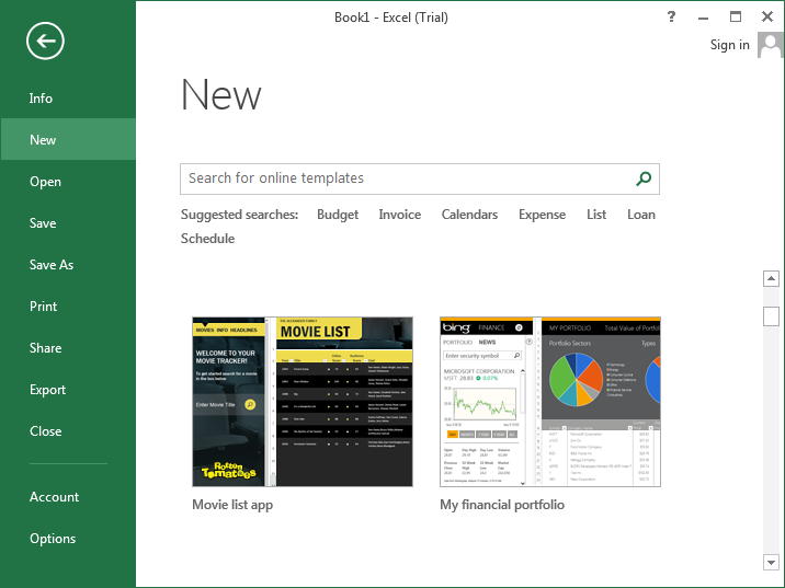
Users who have limited or no experience working with Microsoft Excel will especially benefit from the template options, while regular users will appreciate the “Recent” file list along with hassle free access. Note that while the Start Screen presents a host of benefits, you can even disable it if necessary.
To disable the start screen in Excel 13, open a new document and go to “File”, followed by “Options”. Unselect “Show the Start Screen when this application starts” in the “Start up options”.
Recommended Charts – How to Select, Insert, and Format
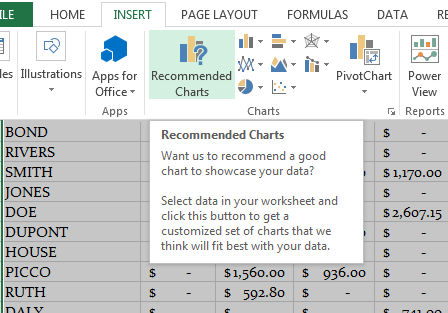
Next the “Recommended Charts” new feature in Excel 2013 illustrates the fact that while fresh features have been incorporated in Excel 2013, they do not meddle with the usability. Basically this intuitive option displays just the breakup of chart types that maybe relevant to the information you have entered in Excel. So even if you are not good with making charts, this feature will help you find the most suitable one without barging in the whole screen.
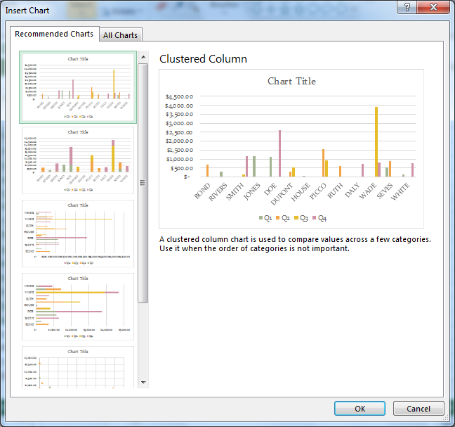
Here in this Excel 2013 Tutorial, we show how you can use this tool. Highlight the information that you want to work on in MS Excel 2013. Next, click “Insert”, followed by “Recommended Charts”. You will now see a dialog box on the screen which has all the chart options. If you click on a chart, you will have a preview of how the data will appear on it. To create a Chart, simply click “OK” and your work will be done.
If you remember from the earlier Excel versions, selecting a chart would make 3 extra tabs appear in the Chart Tools tab. These were Design, Layout, and Format. Now you only have the Design and Format tabs which make the interface of Excel less cluttered. Not to mention, you will also have an additional set of icons on the top right corner of the chart you select.
These related buttons in Microsoft Excel 2013 are “Chart Elements”, “Chart Styles”, and “Chart Filters”, and pressing them enables you to use extra formatting options. For instance, by using “Chart Elements” you can add or remove elements like axis titles, whereas with “Chart Styles” you can change the color of the chart. Finally, filtered data can be viewed with live preview via “Chart Filters”.
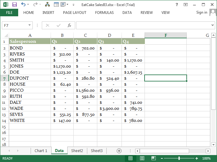
The next three graphic images illustrate how Recommended Charts can be beneficial in quickly analyzing Sales by Quarter information for your team. The first image simply has the data for each quarter by our Sales staff.
Pivot Tables – How to Insert them?
Next item in this Excel 2013 training article is Pivot Tables. These tables are a great feature to help experienced users analyze their data. Note that if you if have not used Excel previously, you will find it hard to create Pivot Tables. However, Excel 2013 has the “Recommended PivotTables” option to get you started. Here is how you can use this option.
Select the entire data (headings included), and then do the following:
Select “Insert” > “Recommended PivotTables” You will now see a dialog box that displays a sequence of PivotTables that analyze and explain the data. To create a PivotTable automatically, simply click “OK”.
Backstage View – How to View and Pin Files
The Backstage View was first launched in Office 2010. To access it in Excel 2013, simply go the File menu. Note that this feature has been improved in Excel 2013 to help you select the correct task. You can even view your recently used Exel workbooks from the “Open Tab” which serves the dual purpose of the “Open” and “Recent” options in the 2010 version of Excel.
You can pin frequently used worksheets to this list and you can click “Computer” to access and pin recently visited locations. You can even access your SkyDrive (online storage), plus add other accounts for cloud storage as well.
Quick Analysis – Use This Tool to Format your Data
We move on to Quick Analysis as we continue with this Microsoft Excel 2013 training. Here is another tool to help you work smoothly on MS Excel 2013 by helping you look for formatting options to use on your data. This is how you can enable the Quick Analysis tool. Highlight your data, and you will find the Quick Analysis icon in the bottom right corner of your data. When you click the icon, a dialog will come into view that will display a variety of tools such as “Formatting”, “Tables”, and “Sparklines”.
These tools will help you analyze the data in MS Office Excel. If you click on these options, another sequence of functions will come into view and you can preview each one by hovering the cursor over them. If you want to use any of the options, simply click on it. This makes tasks like formatting or adding formulas speedier than before.
This is shown from the following screen capture in Excel 2013.

Related Resources on Excel 2013 Training
– Free MS Excel 2013 Tutorial
– Training courses for Excel
– 10 New Features in Microsoft Excel 2013 – YouTube
– Try Office 2013 video training for FREE!
Flash Fill – How to Add or Extract Data
Flash Fill is perhaps the best new tool you will find in Microsoft Excel 2013. The Flash Fill new feature identifies patterns that you use regularly and then adds or removes data automatically in the same sequence. Using Flash Fill in Excel 2013, you can manage some common problems that are not easy to come around manually. For instance, let’s say you have a list of American cities with the name of the state alongside. However, you have to extract just a city’s name from the column.
Simply go the next blank column along with one that contains both the city and its state, and type the city’s name. Next, click “Home”, followed by “Fill” and “Flash Fill”. The blank column will now display just the names of the city. In the same way in Excel 2013, you can add or extract contact details of people, and even extract specific numerical data from the cells. Of course, you can do this with formulas as well, but the Flash Fill makes the process simpler and quicker.
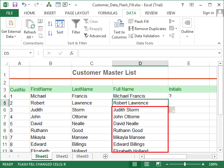
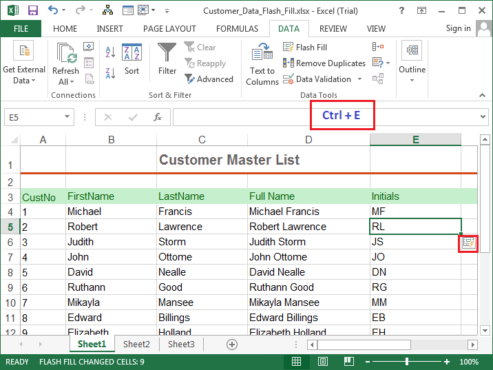
Here in this Excel 2013 tutorial, we have an example of Flash Fill, Excel 2013 new cool feature in Action. We have a list of customers with first and last names. We would like to do the following:
- Combine the first and last name into a Full Name – Column
- Extract the Initials from the Full Name – Column


Power View – How to Create Quick Analysis for Sizeable Data
Next in our Excel 2013 lesson, we are going to look at Power View. Excel 2013 retains the Power View add-in from its predecessors. This add-in is basically utilized for analyzing large chunks of information that has been added via external sources. Power View therefore is a great resource for creating reports in large organizations. To see this tool in action, select the data you want Excel to analyze and then choose
“Insert”, followed by “Power View”.
Note that when you use this for the first time, the Power View installs automatically. Next, a Power View sheet will be added to your Excel 2013 workbook, creating an analysis report on the data you selected. Once the report is created, you can add titles, filter the data, and change its display. To access format options, go to the Ribbon toolbar and select the Power View tab. You will find options like “Theme and text” formats, View options, and Filters Area.
This is what Power View in MS Excel 2013 looks like.

How to Create a Sample Spreadsheet
Considering all the information given above, here is how you can create a basic workbook or spreadsheet on Excel 2013.
To create a new Excel workbook, go to:
File > Click New > Blank workbook
To enter data, you need to click on cells, which are arranged according to their location in row and column. For example, A3. Once you click on a cell, enter text or numerical data and press the Enter or Tab to proceed to the next cell.
To add numbers on your sheet, select a cell on the right or beneath the numbers that have to be added. Select “Home” followed by “AutoSum”. Alternately, you can use the keyboard shortcut Alt +=. Moving on, when you type in = in a cell, Excel recognized that this cell will contain a formula. Using other signs like +,-,*(for multiplication), and / (for division), you can simply press Enter to get the results on any sum. To keep the cursor active on a particular cell, press Ctrl+Enter.
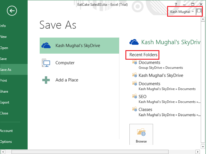
To organize the Excel 2013 data in a meaningful manner, you can use the features mentioned above, such as the Quick Analysis tool and PivotTables. Finally, you can save this workbook on the Web. Sign in to your Microsoft account (Hotmail, Messenger, or Xbox Live). Open the workbook, click “File” and select “Save As”.
Select “Add a Place” followed by “SkyDrive”. Use “Microsoft account” to sign in. Enter account details and click “Sign In”. Now you will find your SkyDrive under the “Places” section. Click “Places”, followed by “Recent Folders”. If you still don’t see your folder, select “Browse for Additional Folders”. Enter the name of your Excel file, and click “Save”.
Next in this Excel 2013 training, lets go ahead and save the EatCake spreadsheet to the SkyDrive that we were working on earlier. If not already signed into SkyDrive yet, you need to click on the Sign In button (top right). After you have logged into you account (get yours at http://www.live.com), you will see a new option. Now you can see option to save to your SkyDrive and even the folders/directories in the cloud. When we tried to save the file, we go the following options:
How to Share your Office 2013 Excel Work
Once you have used to the above-mentioned features to organize your data, you can share your work with colleagues and friends in real time, which is yet another fascinating aspect of MS Excel 2013. Using the Excel WebApp, files can be shared and worked upon by others through SkyDrive. Note that if 2 people try to perform the same action on one file simultaneously, you can experience some problems.
Moreover, if someone else is working on a Microsoft Excel worksheet, you cannot open it from SkyDrive on your device. This limitation ensures that there are no conflicting changes in the same file. However, if an Excel file that is stored online is being used by someone, you can (with permission) download or view it. But none of the changes you make will be reflected in the original file which will remain locked unless the other person closes it.
Also remember that the new Excel 2013, like all other applications in Office 2013, automatically saves files to the cloud which you can access through the a browser with the Excel WebApp even if you do not have Excel on your local hard drive.
Moving on in this Excel 2013 lesson, you can even share files via social network direct from Excel 2013. To share your files on networks like Facebook, start by saving them to SkyDrive first. If you haven’t done so, simply click “File” followed by “Share”, and then select “Invite People”. In this way, you will come across “Save As” options in a while.
After this process, you will return back to the Share panel where you see “Post to Social Networks”. You can choose any social network provided that it is linked with your Office 2013 account. Here you can include a message and decide whether others can edit the worksheet you are sharing. After doing this, your post is ready to be shared.
You can even share Excel 2013 sheets in online meetings. Even if you are not at work, you can simply connect and share workbooks using a smartphone or tablet. However, you need to have Lync installed on your device. To use this feature, first close down any files you do not want to share. Next, click “File” followed by “Share”, and “Present Online”. Finally, click “Present”.
If Lync is not running, you have to sign in to continue. In the “Shared Workbook Window” section, select between a planned meetingor “Start a new Lync meeting”, followed by OK. You can bring in more people to the online meeting by clicking the “Participants” button and selecting “Invite More People”. You can select contacts from the list or enter their names manually. If you need to stop sharing with Lync, simply click “Stop Sharing” at the top of the Screen.
These were the major functions you can perform on the Excel 2013.
Excel 2013 Tutorial – Related Links:
For those who require additional training on MS Excel 2013, then the following links may be good ones to check out:
–What’s new in Excel 2013
–Securing documents in Office 2013
–10 Awesome new features in Excel 2013
–Microsoft Excel 2010 Tutorial
If you are after getting more information about Excel 2013 then the link below is a useful one to look into.
http://office.microsoft.com/en-us/excel/
Connect with US!
![]()